Sensitivity analysis
Although this is simple, it is one of the most powerful techniques available to analysts. Sensitivity analysis involves the running of models with different inputs, allowing their effects on results to be assessed. This provides guidance on the importance of various input factors, allowing you to make decisions on suitable inputs.
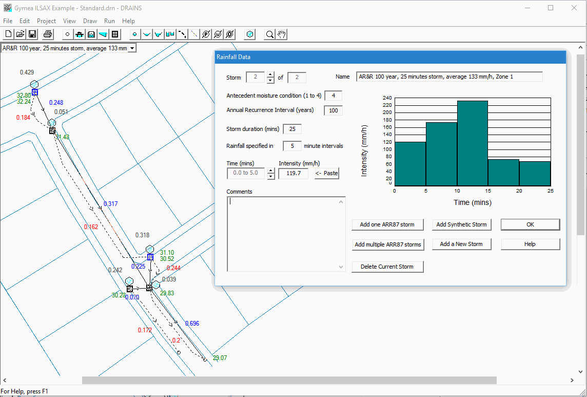
As an example, consider the effects of selecting different values of the antecedent moisture condition in a model. Major storm results from one of the demonstration models, the Gymea Pipe Drain example, are shown below. These are obtained with an AMC of 4, established in the Rainfall Data.

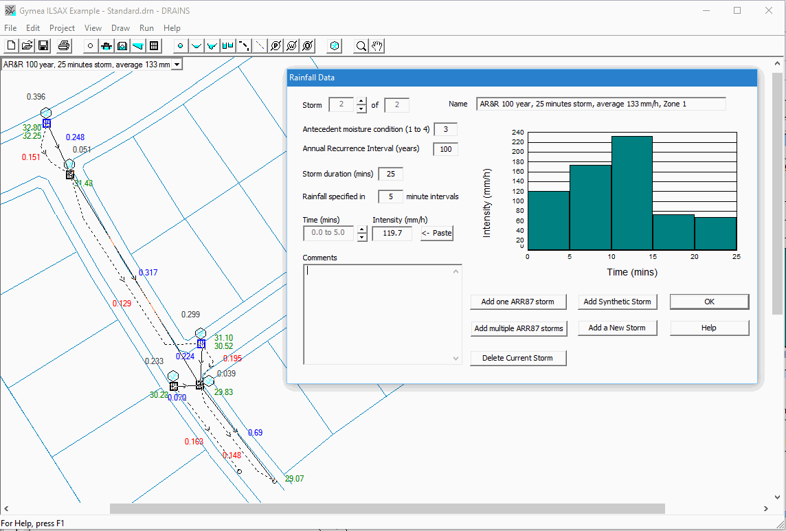
Now consider what happens when the AMC in the Hydrological Model is changed to 3, 2 or 1. The results for an AMC of 3 are shown below.

The major storm peak runoff from the sub-catchments changes as follows:
The effect of the AMC and of the percentage impervious (paved + supplementary) areas in sub-catchments is apparent. The information from the various runs can be used to select an appropriate value of parameters, and to point to factors for which more information is needed.
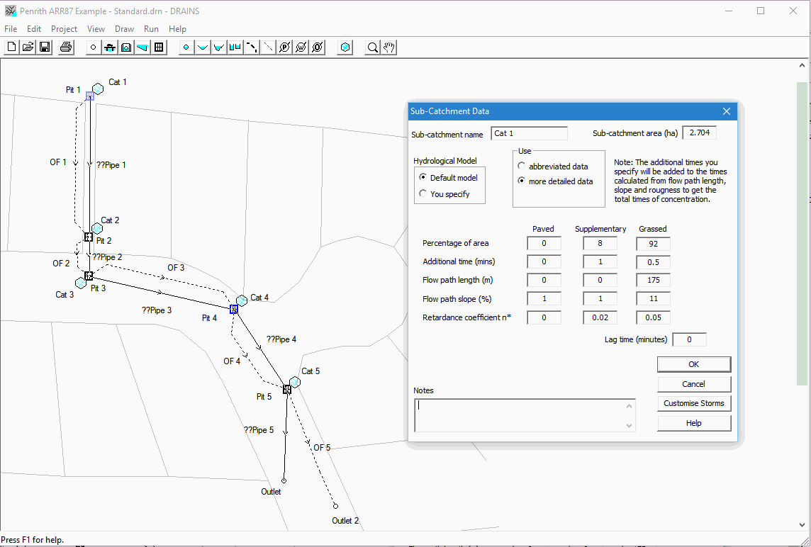
Another example concerns times of flow calculated using the kinematic wave equation. A result from the demonstration example for Penrith is shown below:

As an example, consider the effects of selecting different values of the antecedent moisture condition in a model. Major storm results from one of the demonstration models, the Gymea Pipe Drain example, are shown below. These are obtained with an AMC of 4, established in the Rainfall Data.
Now consider what happens when the AMC in the Hydrological Model is changed to 3, 2 or 1. The results for an AMC of 3 are shown below.
The major storm peak runoff from the sub-catchments changes as follows:
| Pit | % Impervious | Flow for AMC = 4 | Flow for AMC = 3 | Flow for AMC = 2 | Flow for AMC = 1 |
| Pit A.1 | 35% | 0.429 m3/s | 0.396 m3/s | 0.336 m3/s | 0.272 m3/s |
| Pit A.2 | 80% | 0.051 m3/s | 0.051 m3/s | 0.049 m3/s | 0.048 m3/s |
| Pit B.1 | 55% | 0.318 m3/s | 0.299 m3/s | 0.270 m3/s | 0.238 m3/s |
| Pit C.1 | 60% | 0.242 m3/s | 0.233 m3/s | 0.216 m3/s | 0.191 m3/s |
Another example concerns times of flow calculated using the kinematic wave equation. A result from the demonstration example for Penrith is shown below:
Examination of the spreadsheet example for Sub-catchment Cat 1 shows that the grassed area time calculated in a 100 year ARI, 20 minute storm is 7.74 minutes for the surface roughness or retardance of 0.05 assumed in the Sub-Catchment property sheet shown above. If this roughness is varied, the times are:
| Roughness or Retardance, n | Time (minutes) | Peak Flowrate (m3/s) |
| 0.25 | 19.51 | 0.642 |
| 0.1 | 11.47 | 1.01 |
| 0.05 | 7.74 | 1.15 |
| 0.02 | 4.68 | 1.27 |
| 0.01 | 3.26 | 1.28 |
The time of flow, or time of concentration, changes considerably when the roughness is altered, and the calculated flows also change, due to changes in the speed with flows from different parts of the sub-catchment concentrate at the outlet. With this knowledge of the effects of the adopted flow path roughness, and appropriate roughnesses for different surfaces, you can make a judgment on a suitable value.
With the complexity of the results obtained using ARR 2019 rainfall ensembles, sensitivity tests are an essential way to compare different hydrological models and model parameters.
Related Articles
Hydraulic grade line analysis
This is a form of hydraulic analysis of piped drainage systems that traces the positions of hydraulic grade lines throughout the system. It is usually applied as a steady state model, calculating HGLs for the peak flowrates at each pipe in a system. ...Design and analysis procedures
Different design and analysis methods are recommended by the 1987 and 2019 editions of Australian Rainfall and Runoff. The 1987 Procedure The 1987 procedure simulates the conversion of (a) rainfall intensities to peak flowrates, using the rational ...Analysis runs
(a) General Analysis is the main mode of operation of DRAINS, in which the program performs a simulation of the operation of a drainage system during some rainfall-induced event or events, but does not change any aspects of the system that are ...ARR Design and Analysis Implementation
Analysis procedures using rainfall-runoff models are discussed briefly in Section 5.9 of Chapter 5 of Book 2 of ARR 2019. Urban stormwater drainage is not specifically considered, and an example provided in Section 5.9.10 relates to a rural catchment ...Soil type
Soil types used in the Horton (ILSAX) hydrological model in DRAINS follow the U.S. Soil Conservation Service system adopted in the ILLUDAS model from which ILSAX was developed. There are four soil types involving different infiltration ...